
A brief overview of climate dynamics (and how we try to predict changes)

A general transcript of the 16 April 2026 presentation to CA-WN by Dr Colleen Golja.
_____________________
Preface by CA-WN
Planet Earth sits in the infinity of space, powered by our sun, a nuclear reactor 150 million kilometres away.
Since day one, roughly 4,600,000,000 years ago, geological processes and sun-driven lifeforms began weaving an infinitesimally thin security blanket around Earth, a blanket of atmosphere without which Earth would be as habitable as many other planets.
For centuries scientists have been trying to understand how it all works - atmosphere, climate, weather, drought, flood, storm and doldrum - and how records might inform Earth’s future.
In April CA-WN was privileged to be given a talk by climate scientist Dr Colleen Golja, a visiting by-fellow at Churchill College Cambridge and independent Research Fellow within the Grantham Institute for Climate Change and the Environment at Imperial College London.
In the following, Dr Golja provides us with the atmosphere basics, an outline of modelling the mechanisms that drive Earth’s climate behaviour, and introduces us to her own research interest in predicting future climates using mathematical and numerical representations of all the physical, chemical, and biological processes involved.
_____________________
Contents
1. Earth’s Atmospheric Structure
2. Tropospheric Circulation
3. Stratospheric Circulation
4. Patterns of Atmospheric Variability
5. A primer on Climate Modelling and Prediction
6. Future Projections and Change in the UK
_____________________
1. Earth’s Atmospheric Structure
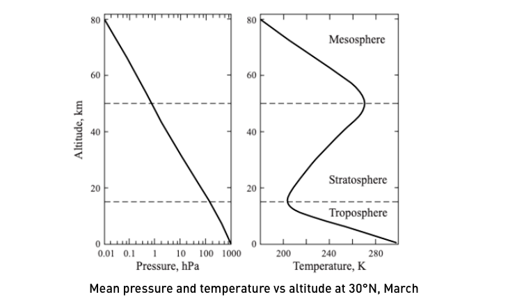
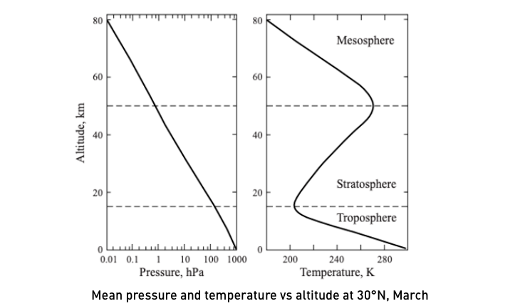
The left of this diagram shows how pressure changes with altitude, the higher in the atmosphere, the less dense. On the right in the diagram, how temperature changes with altitude.
Troposphere
In the troposphere, the temperature gets colder as you go up in altitude until the inflection point between the troposphere and the stratosphere from where it starts to get warmer. [Note that the temperature at zero in the Kelvin scale is minus 273.15°Celsius, absolute zero].
Stratosphere
A layer of ozone causes the increase in the stratosphere’s temperature. Ozone particles absorb energy from the sun and vibrate to create local heating and a temperature inversion that ends up being important for describing all of Earth's atmospheric circulation.
Mesosphere
Beyond the ozone layer, entering the mesosphere, the temperature decreases again. Of relatively little mass, less is known about the mesosphere but it may have a significant impact on atmospheric science. Less studied, it is an area ripe for future research.
2. Tropospheric Circulation
Atmospheric circulation is the large-scale motion of air which, together with the ocean circulation, is responsible for redistributing thermal energy from the tropics to high latitudes, and ultimately to space. It is, at its root, driven by the uneven heating of Earth’s surface by the sun.
Considered as a most basic conceptual energy balance, the Earth is a blob absorbing some amount of the heat from the sun with the rest going into space. Those three things must be in balance - incoming heat must equal outgoing heat plus the amount of temperature adjustment at Earth’s surface.
From that very basic perspective, atmospheric circulation can be thought of as a little box model. The motion of air in the atmosphere comes from the uneven heating of Earth's surface that varies seasonally, with much more heating in the tropics and far less at the poles.
As a basic concept, a warmer air parcel is less dense and will rise in comparison with a colder denser air parcel. That’s the basics of the circulation in the lower part of Earth's atmosphere; the tropospheric circulation.
More of the sun's energy reaches Earth’s surface in the tropics. At the equator, warmed, less dense air rises and as it cools, flows towards higher latitudes, then flows back down to the tropics, then heats again in a convective cycle that creates a kind of convective cell.
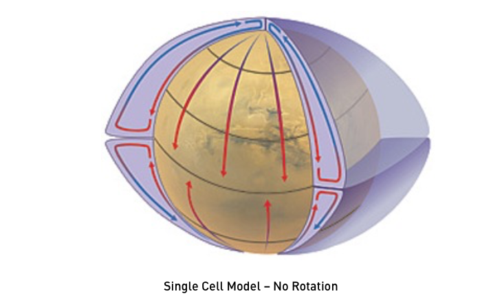
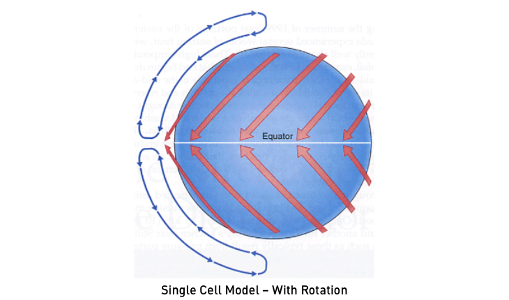
If the Earth wasn't spinning, things would stay in a straight line. But this one cell model needs expanding to including Earth's spinning effect, the Coriolis effect. As circulating air comes back towards the equator it’s being pushed to the left producing an east to west flowing motion. That's interesting in the context of historical sailing routes that took advantage of these typical wind patterns to travel across the Atlantic Ocean.
In reality there isn’t just one cell that is part of this circulation. There are in fact three sets of cells, each related to the total amount of energy received and how far that air parcel travels before it sinks and travels back towards the equator. To maintain the circulating motion in these cells there must be a relatively strong temperature gradient between each end.
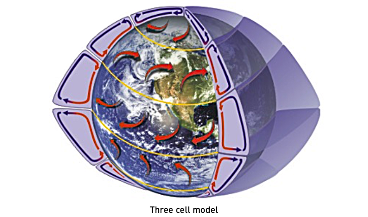
The first cells, called the Hadley cells, take very warm moist parcels of air from the large tropical oceans. This rising wet air, as can be imagined, is essentially getting freeze dried and falls out as precipitation.
The Intertropical Convergence Zone, ITCZ, is the region with these strong rainfall bands. On land, this is where there are rainforests, where rising warm moist air parcels lose their moisture before moving away and descending again. The Amazon rainforest is very much impacted by the ITCZ .
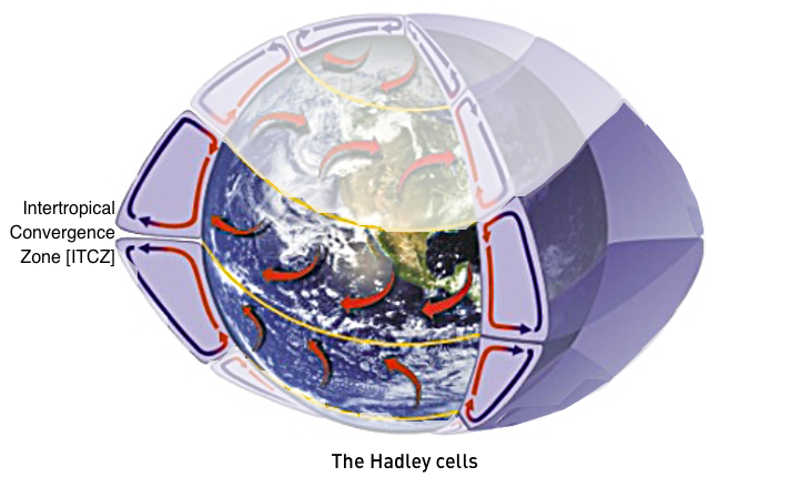
At the other end of the Hadley cells are regions that are on the edge of being wet or dry. Around the globe, the ITCZ has a north-south-north traverse as the seasonal sun strength differs at the equator. The Sahel region across north Africa is the northernmost extent of the ITCZ's traverse. If for some reason that seasonal traverse doesn't reach the Sahel, then the rainfall doesn't reach it. Prolonged changes to the traverse end up causing droughts and that region is particularly susceptible to food insecurity.
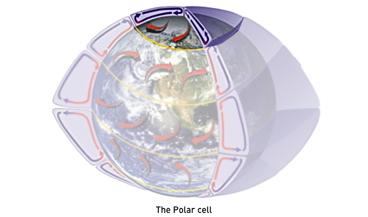
At the pole is what could be similarly described as a thermally-driven cell, the Polar cell. At roughly 60° north, warmer air rises, cools, and then sinks.
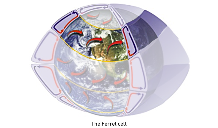
If the Hadley and Polar cells are thermally-driven cells, what is driving the in-between cell? It’s almost as if the air is being pushed like a gear between two other moving gears. And because of that frictional force, and these eddy turbulent forces, a kind of mechanically driven cell is created there. For quite a long time this driving force was not the most well understood piece of the circulation system, and naturally so, because it's not a particularly intuitive explanation.
The thermally direct cells - hot air rising, moving, sinking - the Hadley and Polar cells, are directly moving thermal energy into kinetic energy, between which is a thermally indirect cell. This middle cell is the Ferrel cell, also where colder air rises and warmer air sinks in a way that seems quite odd, but is made possible by this eddy turbulent driving force, a mechanical force. This is particularly interesting for us because this tends to steer where the weather in Europe and North America happens.
The region where the Polar and Ferrel cells abut each other is where many different kinds of air masses collide to create a region of strong winds, the Polar Jet Stream, something that really impacts the UK, sitting above earth at about 9 to 12 km, around 60° north. That's quite far north and in the wintertime, when the equator to pole temperature gradient in the stratosphere is at its strongest, the speeds of this Jet Stream can go up to 300 km/hour. Flying from the UK to North America can take a lot longer than from North America to the UK because of the Jet Stream. In one direction aeroplanes are pushing against the airflow, in the other aircraft are being pushed quite a bit faster.
The Jet Stream dictates where regions of rainstorms will happen. In a year when the Jet sits squarely over the UK, that's typically a year of increased storminess. The reason that it moves and is not completely stationary in one spot is because of waves - Rossby waves - that make the Jet Stream wiggle.
Think of the atmosphere as an ocean of air with disturbances that cause wave structures just like waves in the ocean. And if a wave ripples like a ribbon, that ribbon will wobble. If it wobbles northwards it will bring warmer tropical air over the UK, and if it wiggles southward it draws cold arctic air down over the UK.
In the United States there have been situations where the Polar Jet Stream dips so far south that it brings really cold arctic air in places where typically it wouldn't be expected. A vortex forms a little bit above the Jet, sometimes called a Vortex Outbreak, a cold air outbreak; the polar Jet dipping is the mechanism through which this happens.
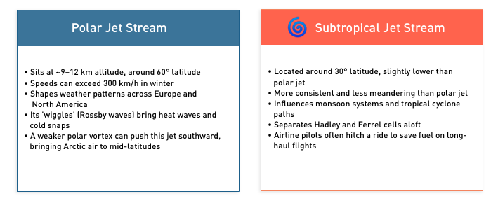
There's also a Subtropical Jet Stream which sits about 30° between the Hadley cell and Ferrel cells. It's more consistent, less impacted by wave breaking or wave ripples flowing through the atmosphere, and typically influences monsoon systems and cyclone paths. It firmly separates both of those cells aloft, and again, is where airline pilots can predict, or try to predict, its location so they may fly in that region of higher winds.
Right now a lot of people are using AI models to try and better predict where pilots can fly the most optimally efficient route through these Jets to take advantage of the wind patterns.
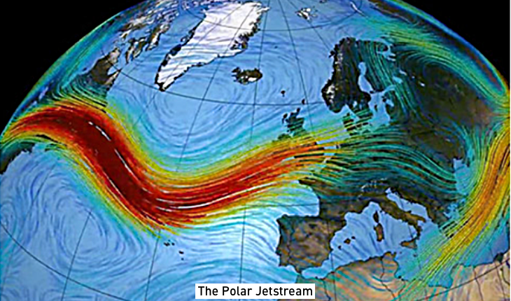
This image from the Met office shows the Polar Jet wind and its meandering pattern directly over the UK. Its obvious wobble has cold air sitting northward and is separating a region of much warmer air further south, meaning the UK will probably get quite a bit of rain, windiness, and possibly storms. Now, in the context of climate change, we can begin to understand that the UK is quite impacted by the position of the Polar Jet
Also, in the context of climate change, people are using the term arctic amplification, meaning that the Arctic areas are warming faster than other parts of the Earth. This means that instead of maintaining a large temperature difference between the tropics and the poles, the poles are warming faster and the temperature gradient is getting less.
Diminishing temperature differences between tropic and pole means weakening Polar Jets, and a weaker Polar Jet is more susceptible to wobbles or waves in the system. With more wobble comes a less stable separation of Arctic and more southern tropical air. It’s assumed there will be greater variability in temperatures in the UK because of increased Jet stream wobbles; sudden changes bringing outbreaks of either cold northern air or warmer southern air.
What's interesting in the context of climate modelling is that it's very difficult to capture historical observations of the Jet so there’s not the most robust ability to predict future changes. While there's a basic mechanistic understanding of what would happen, quantifying where the Jet might more typically lie or what the wigglier Jet might look like is actually quite difficult.
Part of that has to do with other parts of the Earth's system that affect the Jet - which is next.
3. Stratospheric Circulation
The stratosphere has quite a big impact on the strength and wobbliness of the polar Jet, as does the equator to pole temperature change.
The tropospheric circulation is Earth’s more turbulent atmospheric region, where all weather happens. It's where we live, and where people have focused on climate change because that's where all the surface impacts occur. It’s only in the past decade or so that has there been recognition of the importance of including the stratosphere in climate modelling to fully capture surface climate behaviour.
The stratosphere gets warmer as it gets higher. Therefore it doesn't have the same convective overturning dynamical system because the colder, denser air at its lower levels doesn’t want to rise to the warmer air above it. For a long time people assumed that the stratosphere was stationary, that it wouldn't necessarily have a circulation.
Extremely low levels of water vapour were being detected. Higher latitudes are much drier, and the stratosphere is extremely dry. There was a question, how is water vapour moving from the tropics to higher latitudes? This prompted the answer, it must be possible to move material in the stratosphere from the tropics towards the poles. But what would be the mechanism?
It turns out that the stratosphere is actually a wave-driven circulation. It is in radiative equilibrium and there are waves breaking in the stratosphere that push it away from this equilibrium and move material mechanically from the equator to the pole - which was really quite a cool discovery. In fact, this tropical region is known as the surf zone. It can be imagined as being like an ocean with waves crashing, which in three dimensions is a little bit challenging when we are used to looking at the actual ocean where we see waves crashing on a horizontal plane. When a wave breaks, its momentum pushes material. There is a role for the mesosphere here. It modifies with a different type of breaking wave, gravity wave breaking, and smaller Rossby waves, sometimes called Planetary waves.
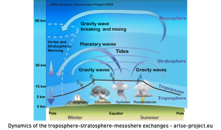
In the stratosphere, because air isn't necessarily rising as a function of the temperature, there’s a really interesting way that material gets into it. One of the biggest sources of small particles, sulphate aerosols, are put into the stratosphere by volcanic eruptions where the explosive energy of the volcano pushes material up into the stratosphere. Once it's there, wave driven circulation moves it throughout the entire stratosphere. As a single cell system it's quite good at moving material from the tropics to the poles, taking about 2 years. It's relatively slow, but once sulphate aerosols are there they are retained for quite some time.
It had been understood that the water vapour in the stratosphere comes from the rising warm moist air from the tropics, decreasing in temperature as it rises before being freeze dried out, with whatever water managing to make it into the stratosphere setting the water vapour budget for the whole stratosphere.
Now, within the atmospheric science community, there's an increasingly held concept of ‘convective overshoot’; a really strong thunderstorm with so much energy that the air parcels themselves become so out of balance with the air around them that they'll overshoot into the stratosphere, inject water and then come back down.
Researchers are currently trying to quantify how much water vapour might be entering the stratosphere through that pathway. It's quite interesting, and still relatively unknown because it's hard to quantify. There are some historical measurements of the stratosphere, so there’s some idea of the temperatures, and there’s an idea of how much water vapour is there.
Once it was discovered that there was an ozone hole there was an obvious interest in understanding the ozone layer, but until then, there was no interest. Therefore, there’s a relatively short observational time series of its constituents. The stratosphere is something that researchers are investing in and now starting to understand.
One of the key features of the stratosphere is the stratospheric polar vortex, something like a stratospheric sister to the polar Jet Stream. Areas in the atmosphere are delineated as one mass of air, such as a strong polar vortex, usually a wintertime vortex in polar night sitting above the polar Jet Stream.
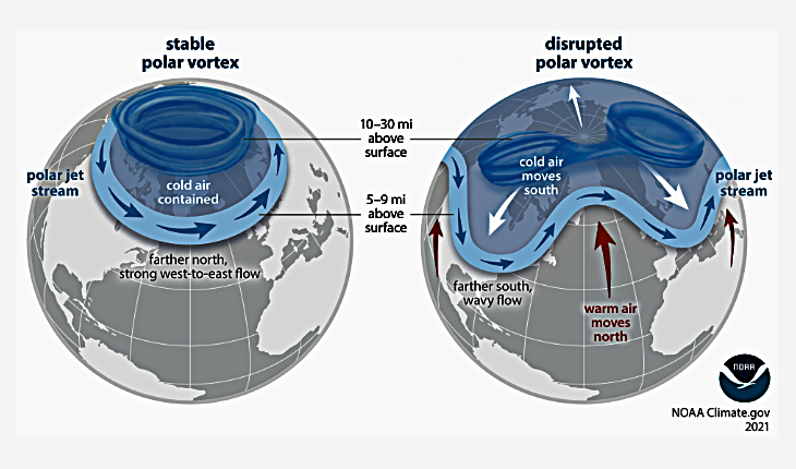
The image on the left shows a 3D vertical structure and what's quite interesting is that you can get these disruptions to the vortex which are again wave-driven. If there’s a really large disruption that rises into the stratosphere it can break the vortex into two chunks, as the image on the right. It can be visualised by imagining a spinning vortex in a water tank. Shaken enough, it could probably be broken into two spinning bits. Once the vortex is broken it cascades down into the troposphere and can disrupt the Jet Stream too.
For example, North America in 2021 suffered a sudden stratospheric warming - so called because when disrupted in this way, there’s a massive temperature change in the stratosphere, which is normally quite cold, but suddenly becomes exceptionally warm before coming back into equilibrium. In 2021 the polar Jet was pushed so far south that it was over Texas, and was called the Texas freeze. It was an insane event; toilets froze in Austin, Texas, and the city was obviously not prepared for this type of weather anomaly. It caused millions of dollars of agricultural damage.
These events are really hard for scientists to predict so no one had time to prepare. When we do future predictions, trying to understand how extreme events might change, understanding changes to the stratospheric polar vortex and the polar Jet Stream is a huge area of research.
Do we expect there to be more of these disruptions because of changes to the structure? Does that translate to more extreme events at the surface like these freezing events that would impact the UK in the same way? The UK is prepared a little bit in both directions. It can handle a little bit warm and a little bit cold, but maybe not a lot warm or a lot cold. This is something worth considering, worth researching the mechanics of how these things break down.
4. Patterns of Atmospheric Variability
There is the ever-ongoing general circulation pattern, and there’s a relatively reasonable idea of what that should look like as it varies seasonally. Then there are patterns of atmospheric variability, recurring large scale shifts in pressure and circulation. These dictate regional weather and climate for weeks, even decades. Probably the most famous is the El Niño southern oscillation, an oscillo-climate feature, with its La Niña counterpart oscillation.
Most relevant to the UK is the North Atlantic oscillation (NAO) and a very similar pattern in the southern hemisphere, the Southern Annular mode. These modify regional and global temperature precipitation and storm tracks. The North Atlantic oscillation is probably most relevant to the UK.
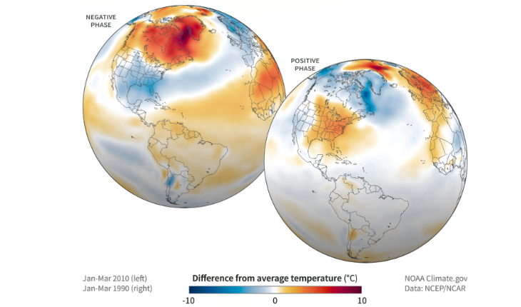
During the negative phase, on the NAO image left side, there is a positive temperature anomaly over northern North America, Canada and Greenland. At the same time there is a negative temperature anomaly over the UK. The right image shows the positive, inverse phase, a cold anomaly over northern North America and a warm anomaly over the UK.
From an air mass perspective this can be visualised as if a toilet plunger was placed on the top of the Earth at the North Pole and pushed down. It would push the air mass south. It would flow so there’s less air over the North Pole, and more air south of 30° north. Pulling the plunger up pulls mass back up and over. In this way, air that is sloshing northward then southward changes pressure, and ends up dictating differences in sea level pressure as well as the temperature patterns that we now know are indicative of that particular oscillation pattern.
Historically this was measured by meteorological stations on two islands where it had been noticed there was a consistent change to the difference in sea level pressure between them. This is now referred to as the NAO index and it can feel quite arbitrary. The difference in pressure is between two box regions; measure the pressure in each, take the difference, then see if that pressure is higher or lower than average. Does that mean this is a positive or negative NAO phase?
In the NAO phase where the pressure is higher there is more air mass sitting over the North Pole, the Jet Stream has shifted north, the air mass has been sucked upward and moves the storm track that comes along with that Jet Stream. Europe then experiences more storminess and precipitation and is typically warmer than average because air from the lower latitudes is being moved up.
During the negative phase, when that ‘plunger’ is pushing down, air is pushed down, the Jet Stream and storm tract have a more west to east orientation and there’s decreased storminess, less precipitation and it's a bit colder in Northern Europe.
So, for each NAO phase there are colder drier or warmer wetter weather patterns. The MET office may say that over this next six-month period we are in a positive phase so you can expect either colder or drier weather.
The NAO wasn't something learned about in school, nor at university. But it has a big impact on everyday weather especially in North America and the UK.
5. A primer on Climate Modelling and Prediction
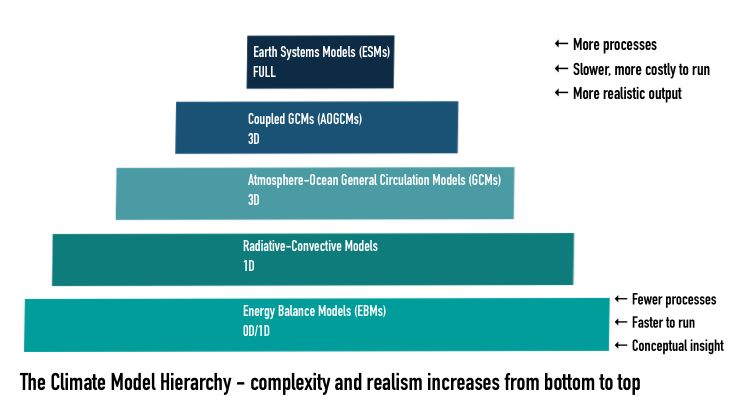
The climate modelling community has a hierarchy of models that are used in the prediction of future climate change. If it’s said that some amount of climate change would be expected because of an increased amount of greenhouse gas in the atmosphere, that claim needs to be backed up with a mechanism describing why that change would take place.
To simplify the processes relevant to that claim, complex models can be coupled with much simpler idealised models.
Energy Balance Models
The least complex climate models are the Energy Balance Models at the bottom of this pyramid. These are the simplest version of the assumption that the energy from the sun is balanced by the total temperature change at the surface of the earth plus the energy out.
As long as energy is balanced, and if the heat capacity of the medium has been understood, then the temperature change can be broadly calculated from how much of that energy has been transferred to the mass and matter in the Earth's system and how much is lost to space.
Planetary scientists will use this type of model to roughly estimate what's often called the skin temperature of the Earth, that would be Earth’s temperature if there wasn't an atmosphere. That could be done for other planetary bodies with an unknown atmosphere, or with only a rough guess of what kind of surface it had.
Radiative Convective Models
Radiative Convective Models combine the movement of mass and energy through a system. The amount of energy coming from the sun is known, as is how much the surface is heated up. A hypothetical column through the atmosphere might be divided into discrete layers. Outgoing energy must move through these layers. The amount of energy a layer absorbs is dependent upon its composition. A layer of mostly ozone will absorb energy and increase the layer’s temperature. These basic mathematical atmospheric models can give a sense of how the temperature changes through space.
Radiative Convective Models can be one or two dimensional. Linearised models replace complex systems of differential equations. Linear approximations of nonlinear systems can solve differential equations more quickly with less computing power but giving up complexity.
General Circulation Models
In terms of climate circulation modelling, either the atmosphere or the ocean is fully described, or there are fully descriptive models, typically of a given part of the earth system, General Circulation Models (GCMs),
An atmosphere/ocean global climate model can represent the full atmosphere and full ocean but may not include sea ice and river runoff. GCMs are fully coupled Earth system models, the most complex versions that represent the full atmosphere and the full ocean. They usually have a vegetation model, a land systems model, river runoff, and sea and land ice. They're incredibly complicated and incredibly expensive to run. So, especially when you're testing new mathematics, the simplest version that can run the test is used before building complexity.
Colleen, currently working with the UK Met Office to update some of the mathematical representations of the fully coupled United Kingdom Earth System Model (UKESM) housed at the Met office, outlined one situation:
‘We changed one small parameterisation that was describing how clouds behave at a particle level. We were saying, "Okay, we actually think that the cloud condensation nuclei might behave slightly differently. Let's update this." And we ended up with a simulated climate that was totally different than we started with. We ended up having to scrap that, go back to this individual atmosphere model, figure out, okay, why did this change our rate of balance so much? Why did this modify how energy is moving through the system so much? Then recalibrate everything and go up through the complexity pyramid back to the top. Instead of being a very short-run project, it was a three-year long project - things can be a little bit more sensitive than expected’.
When they become available, the Met Office integrates new observations into its Earth System Model. As more data become available there has been a move to using machine learning models to compute relationships, statistical models are used instead of calculating certain features from physics equations.
However, this approach is being criticised. With CO2 moving into a new regime that has never been represented in historical observations, how is it possible to apply a statistically learned model to such an out-of-sample situation?
How to gain computational efficiency without sacrificing predictive capability is currently one of the main discussion points in the climate community. Where can these statistical models fit in and where can they not, where should they be used and how should they be understood, that's the real point of the current discourse right now.
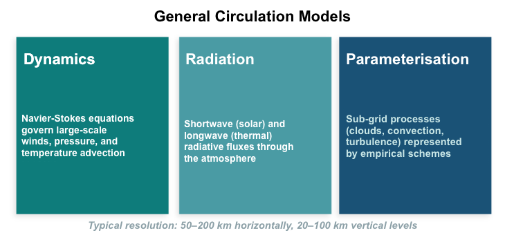
Fully coupled GCMs can simulate realistic weather patterns and Jet streams. They discretise the atmosphere into a 3D grid, or sometimes even a hyper-complicated grid of cells, and at each grid cell or across each grid boundary, they solve equations of fluid motion, thermodynamics, and radiative transfer.
The complaint about GCMS is that sometimes they don't do a very good job. But it can be argued that all models are useful. They do help us learn, though whether or not they are capable of helping us perfectly predict the future is up for debate. But without doubt they are certainly able to tell us that greenhouse gas emissions have driven warming and changes to the climate. However, more work is required to understand exactly how future changes will occur - models need to get more niche with very system-specific regional knowledge.
It is incredible that these massive models are being built. In particular, the area of research on parameterisation. Any process that can't be described because it exists on a scale too small, or on a scale much smaller than the grid scale at which the model itself runs, has to be parameterised. This means, at every time step, there's some kind of empirical equation calculating what it is doing and how it feeds into the bigger spatial domain.
Researchers are thinking that machine learning or statistical relationships can replace some of these traditional parameterised functions. Parameterisations tend to get too convoluted and require excessive processing power to compute. Instead of representing them all, a choice must be made about which parameterised process is most important to include.
If there were a faster way of doing this, then more important processes could be incorporated while maintaining computational tractability. This is particularly important for aerosol cloud interactions. Aerosols are any small particle that stays aloft in the air; dust, sea salt spray, pollen and black carbon. These and other kinds of particulate matter in our atmosphere interact with clouds in very complex ways.
Because clouds can reflect incoming radiation, or lead to local warming, they have a massive impact on how sensitive the Earth system is to a change in carbon dioxide radiative forcing. These cloud aerosol interactions are probably the most pressing area of climate research in the modelling community at present.
It is quite difficult to incorporate ocean circulation into atmosphere research. Typically models are simplified using what is called a ‘slab ocean’. Instead of fully resolving the circulation of the ocean and its energy uptake, oceans are treated as a heat sink. Oceans take a long time to equilibrate their surface temperatures. The study of small-scale atmospheric processes does not necessarily need oceans to equilibrate; a realistic image of their heat flux serves instead. This is unlike an analysis for an IPCC report which does require an understanding of climate sensitivity. The full ocean must be attached and the model run until it hits equilibrium.
Example Earth System Models
The Community Earth System Model (CESM) is housed at the National Center for Atmospheric Research in the United States in Colorado, one of the world’s most prominent places for climate research.
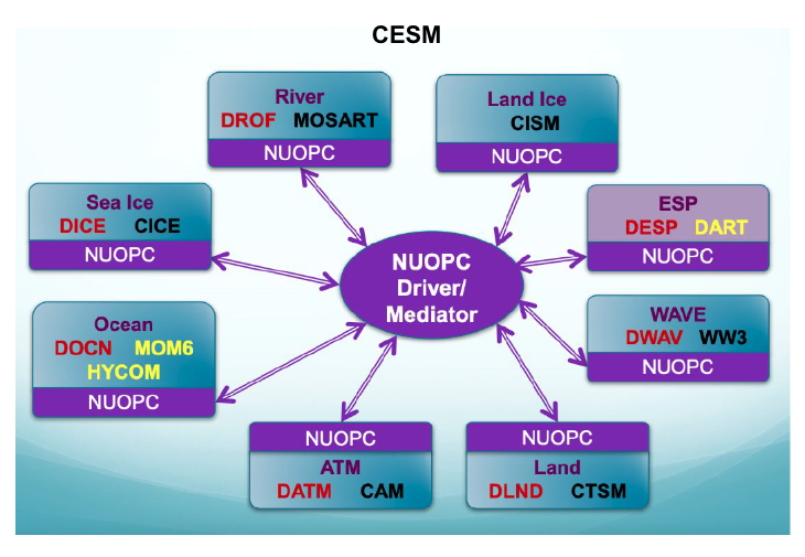
The CESM is community-based and open source, anyone can download it. CESM has community support, a help desk and a help bulletin. Not everyone has the compute capacity to run it but a subset can be downloaded. For example, the CESM atmospheric column model can be downloaded to allow non-scientists to explore it with community support. It is really valuable to have that level of support.
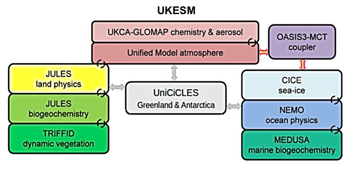
The Met Office’s United Kingdom Earth System Model (UKESM) is also extremely well documented and kept up to date. It has an extraordinary level of detail in its modules that, as the above diagram suggests, provide interactive, two-way feedback with the atmosphere and ocean components of its global climate model.
Its atmosphere module, GLOMAP, is a state-of-the-art aerosol and chemistry module - many other models sacrifice some atmospheric chemistry because it is so complicated and it requires so much compute power.
UniCiICLES is the dynamic ice sheet model that simulates the behaviour of the Greenland and Antarctic Ice Sheets. There are sea ice, ocean physics and marine biogeochemistry modules, land physics, biogeochemistry and dynamic vegetation modules. The dynamic vegetation module models the behaviour of plant life as increased CO2 modifies rates of respiration and photosynthesis. Modules like this enable downstream impacts assessment.
For example, the outcomes for agriculture; researchers take key parameter outputs from models with dynamic vegetation simulation, like UKESM, and feed them into impact assessment models or agricultural models to say that, for example, under these future scenario conditions, soy, corn or maize products will be expected to behave like this. Having all these modules integrated is incredibly useful for evaluating downstream impacts.
6. Future Projections and Change in the UK
Thinking specifically about future projections and changes in the UK, there are different Representative Concentration Pathways - RCP scenarios. Each RCP represents assumptions within a set of possible future climate evolution scenarios, typically a low greenhouse gas emissions scenario, a medium emissions scenario and a high emissions scenario.
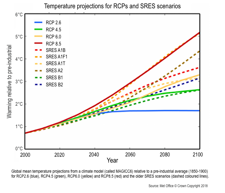
The diagram from a 2018 Met Office projection shows RCP 8.5 in solid brown and SRES A1F1 in dashed brown. These are ‘business-as-usual’ scenarios, where emissions are not cut. These estimated about a 5°Celsius global average surface warming by 2100, which would be catastrophic.
The new IPCC Assessment Report is being informed by a new kind of background emission scenarios, the Coupled Model Intercomparison Project Phase 7, CMIP7.
There's one incredibly enthusiastic and optimistic scenario of a slight temperature overshoot, of emissions being cut aggressively before negative emissions by around 2085.
There's a medium scenario, still with emissions cuts, still with a global temperature increase.
Then there’s an updated ‘business-as-usual’ scenario driven with updated information about our current emissions.
Based upon these three projections, scientists will take the emissions from the RCP scenarios which each feed out CO2 emissions but they also feed out other greenhouse gas emissions such as methane, nitrous oxide and CFCs.
The RCP scenarios also dictate aerosol emissions and aerosols are really interesting. Sulphur dioxide, SO2, is one of the big aerosols emitted from burning fossil fuels, specifically coal power plants and smelting processes. SO2 is quickly oxidized to become a reflective particle that has a strange feature when associated with greenhouse gas emissions; it leads to cooling because it reflects sunlight away from Earth. In 2020 the global community saw reduced sulphur in shipping emissions. These reduced SO2 emissions also reduced this reflective layer which led to a slight temperature increase. The resulting temperature profiles, especially the regional climate impacts, are very dependent on the emissions profile fed into a model - and there's a lot of debate around that.
The UKCP18 report, from 2018, is a bit outdated but the general findings have remained. Under the high emissions scenario it projects a greater chance for hotter drier summers, warmer wetter winters, and more extreme weather. By 2070, winters could be up to 3.4°C warmer and summers could be up to 5.1°C hotter.
What is striking is how much more variable weather could get. A technical paper released since the Los Angeles wildfires talked about climate whiplash, how extreme events on their own are very damaging. If extreme events are back-to-back, like a drought followed by extreme precipitation, then you can get exponentially more damaging outcomes. In a drought for example, because the soil becomes hydrophobic it has less absorption of what becomes catastrophic flooding. With more likely oscillations between extremes, each extreme is made more damaging. This is how many climate scientists are starting to think of assessing extreme events, the assessment not only of the frequency of the extreme, but also how likely it is to be occurring in tandem with another extreme event.
_____________________
If Colleen’s talk has inspired you to learn more about climate change you might wish to read MIT’s Climate Science, Risk & Solutions